
Advanced HTML5 Canvas Techniques – Pixel Manipulation and Bézier Curves
Our last installment on HTML5 Canvas looked into the geometric and algorithmic fundamentals behind the many abstractions over the relatively primitive native Canvas API: we talked about planar point sets, the square lattice, sorting points by polar angle, and convexity detection.
In this third article, we’re going to introduce two more useful algorithms, but we’ll also cover a native Canvas capability we hadn’t gotten around to yet: access to individual pixel data. We’ll demonstrate this with a basic computer vision operation, edge detection. After that, we’ll show a way to go beyond Canvas’ native implementation of quadratic Bézier curves and render higher-order curves.
This is a lot of territory to cover; let’s start things off gently, by talking about pixels and color. As usual, all our example code figures are links to jsFiddle, where you can test and experiment with the code yourself.
RGBA Image Data
Like many foundational graphics APIs, Canvas’ ImageData interface represents colors as arrays of four bytes; one each for a pixel’s red, green, blue, and alpha components. You can construct an ImageData directly or obtain one from a CanvasRenderingContext2D, but we’re going to acquire our initial ImageData from an image DOM element. This will be our full-color source, to convert into grayscale and draw onto the destination canvas. Let’s take a look:
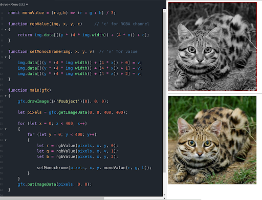
Here, we’ve rendered a source <img> and copied it (by drawing its ImageData) into our destination canvas. Our initial goal is to convert the picture to monochrome. We create a couple of 2D accessor functions because ImageData only provides a one-dimensional pixel array. And we define monoValue() to calculate grayscale values by averaging chromatic components. Our processing loop acts directly on the destination pixel array, but note that the changes aren’t rendered until we repaint the canvas context with putImageData().
Convolution Effects
Convolution is a signal processing technique that derives, from two functions, a new function describing the relationship between them. In image processing, this involves altering each pixel according to some function of its immediate neighbors. Consider the following slight blur effect, which simply sets each pixel to the average value in its 3×3 neighborhood:
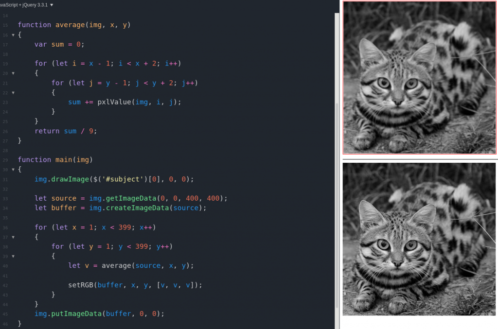
In this example, our convolution operation is average(). The region of pixels involved in the operator is called the convolution kernel. Since we’re just averaging a 3×3 area, our kernel could be summarized like this:
[ 1, 1, 1 ]
[ 1, 1, 1 ] / 9
[ 1, 1, 1 ]
In this abbreviated notation, matrix values are input scaling factors; the value at right divides the kernel sum. Many of the typical filters built into image manipulation software, like emboss or bezel effects, are simply convolutions with different kernels.
A couple details to notice about this code: first, the main loop excludes the perimeter of the image, because parts of the kernel would be undefined there (for kernels larger than 3×3, we’d need a bigger margin). Second, we don’t modify the original source pixels, but rather a copy buffer; this prevents output pixels from interfering with convolution of the remaining input. Blurring is a typical precursor to our next convolution example, the Sobel operator for ‘edge detection.’ This process is more complicated; we use separate kernels for the X and Y axes and then combine them:
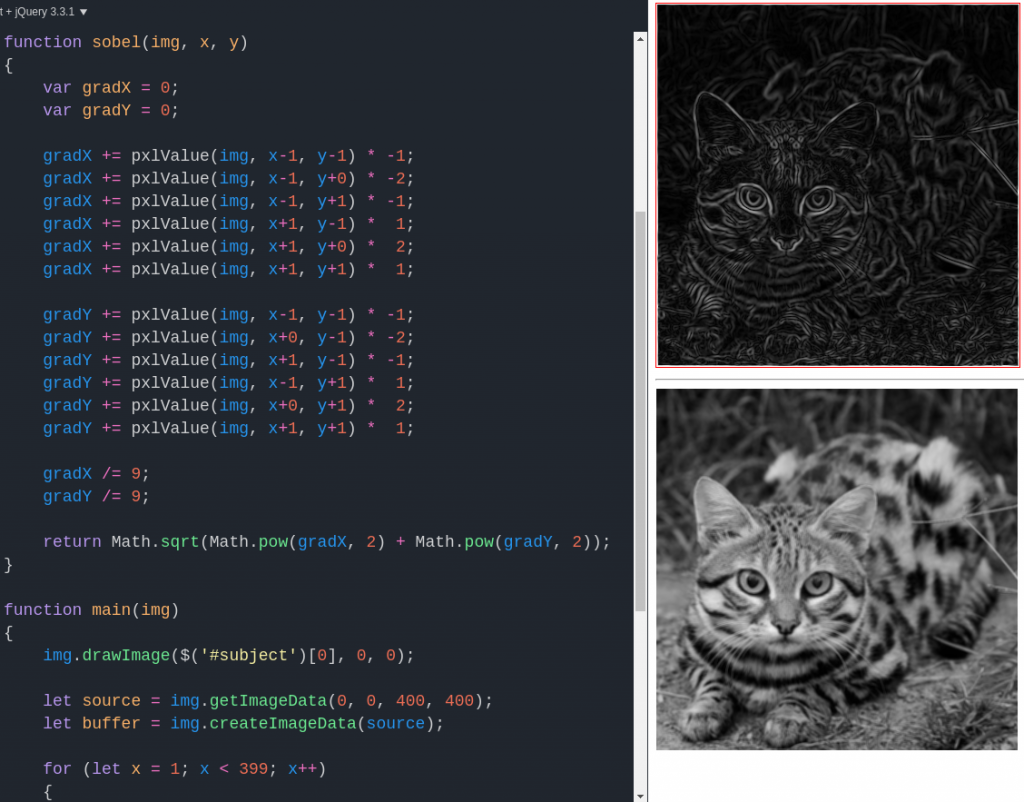
The Sobel operator is a relatively primitive edge detector – as you see, its output is rather noisy even though we’d blurred the input. But more advanced edge detection steps are often early stages in computer vision applications, as the input to a thinning or thresholding process, for example.
Bézier Curves
If you’ve worked with vector drawing applications before, Bézier curves are probably familiar. They’re a convenient way to specify a curve interactively, by dragging around control points that modify the curve’s shape. A quadratic curve, for example, is specified by two endpoints and one control point; Canvas’ rendering context has a native method for drawing these. For higher-order curves, we add more control points; two points specify a cubic curve, three a quartic, and so on.
The algorithm of choice – in terms of simplicity and numerical stability, but not necessarily speed – for calculating Bézier curves is that of Paul de Casteljau. Given a point array (two endpoints, with control points between them), it converts values in the unit interval to points along the curve. Below, we illustrate the standard (recursive) formulation of the algorithm, applying it via currying for added fun:
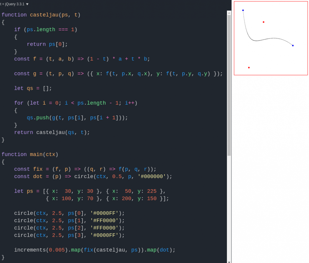
In the output canvas, the endpoints are the blue dots, and the control points are red. This curve is cubic, but we can easily render more complex ones:
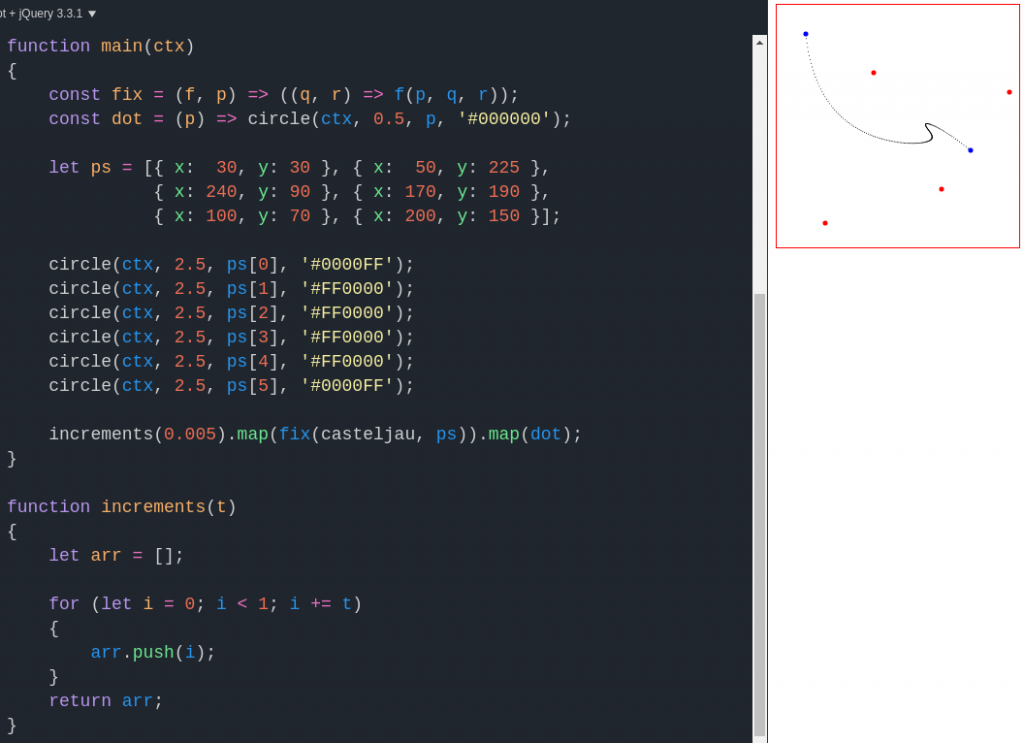
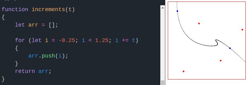
Notice the curve gets thinner near its endpoints – that’s because we applied casteljau() to equally-spaced increments of 0.005 along the unit interval, but the algorithm’s output isn’t always equally dense along the interval. If desired, we could employ linear interpolation to fill in the gaps. Last but not least, note that t need not actually be between zero and one – we can extend the Bézier curve beyond its endpoints:
So with that, we’ll wrap up today’s installment of this series – hope you enjoyed learning more applications of the web’s most advanced 2D graphics API. Thanks for reading, and we’ll see you next time!